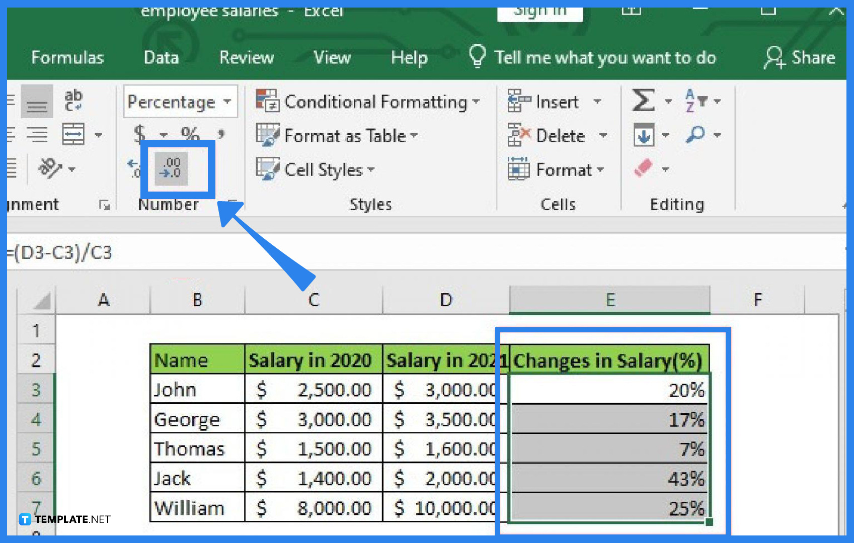
How to calculate p value in excel: step-by-step guide _ calculating p value from f

Schlagwörter:P-Value How To CalculateCalculate P-Value Using ExcelHere’s how to calculate the P-value in Excel by hand: Open the spreadsheet with the data you want to conduct a hypothesis and click on the cell you want to calculate the P-value. Having your data organized and ready in an Excel worksheet will make the process smoother. This formula takes the final value, divides it by the initial value, raises it to the power of one divided by the number of periods, and subtracts one.This is a great tool for data analysts, who can use Excel to calculate the variance using functions like VAR. In the fx tab above the cells, enter the TTEST’s formula =T.Calculate P-value in Excel with Analysis Toolpak. This will collapse the selected rows into a single group, allowing for better organization and analysis of data. For example, to count the blank cells A1 to A5, write the COUNTIF function below: = COUNTIF (A1:A5, “”) The answer to this will be 5 That’s because we have set the criteria blank. Create and populate the table.54% probability that the results could have happened by chance. Since this value is not less than . Now, use the following formula in the cell where you’d like to generate the p-value of the F-test: =F. Perfect for beginners, this guide simplifies statistical analysis for you.Step 5: Press Enter. For example, in the table .Methods To Calculate P-value In Excel. If you’re looking for a specific value, you’ll generally want to set this to FALSE. Example 1: Calculate P-Value for Two-Tailed Test.

How to Make Excel 2010 formulas calculate automatically - YouTube

Begin writing the HLOOKUP function as follows: = HLOOKUP ( B5.The following examples show how to calculate a p-value for a test statistic in Excel in three different scenarios.

How to Calculate P Value in Excel: Step-by-Step Guide (2024)

Enter the compound interest formula in cell A5.TEST(F2:F12,G2:G12,2,2) Calculated p-value . What is the p-value? Measuring the P-value. This gives you the annual growth rate.P (B2:B7) Pro Tip! The STDEV. What is the P Value? P-value is a statistical term that helps you to determine, if the .

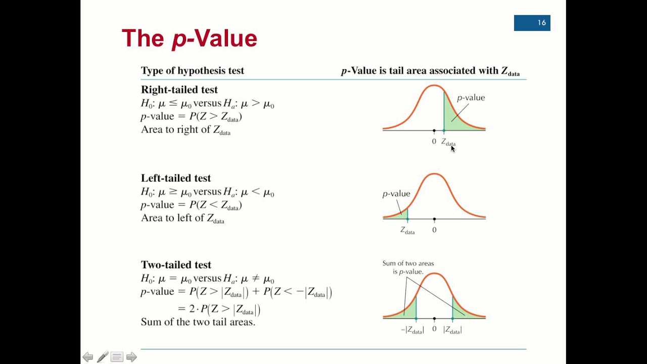
Mastering VLOOKUP in Excel: A Step-by-Step Guide (2023)

P function as follows: = STDEV.Replace “tails” with the number of tails the test uses.The p-value is an important statistic that tells us the probability that the results of our experiment could have occurred by chance. In this tutorial, we will walk through the steps to . To calculate P Value in Excel using the T. The p-value helps to determine the strength of the evidence against the null hypothesis and is a crucial component of statistical analysis.

How To Calculate P-value In Excel

Why is a p-value important? It helps determine . Master essential formulas and simplify your data analysis process today! Skip to content.

P value excel - rasermm

By calculating the p-value, researchers can determine the statistical significance of their findings.Schlagwörter:Microsoft ExcelP-Value Formula A p-value is a number between zero and one. This will open a window where you can select the two samples you want to compare. The range lookup can be set to TRUE for an approximate match or FALSE for an exact match. There are many add-ins available that can perform statistical analysis and calculate P-values . Below is its basic syntax and arguments: =PV(rate, nper, pmt, [fv], [type]) rate: The interest rate of each time range. Let’s walk through calculating a p-value in Excel using the two sample T. nper: The total number of payment time ranges. Remember to use the absolute value of the t-statistic for a less-than test.

How to Calculate Markup in Excel | Techwalla.com

Schlagwörter:P Value in ExcelP-Value How To CalculateMicrosoft Excel

Calculate P Value in Excel

Method 1: Calculating P-Values with T-Test.Just arrange the input datasets of two different samples as shown above.To calculate p-values in Excel, you generally use the T-test statistical function for hypothesis testing.

Demystifying P-Values: A Beginner’s Guide to Calculating P-Values in Excel

Lastly, we’ll use the following formulas to calculate the total positive signs and negative signs and calculate the corresponding p-value of the sign test: The sign test uses the following null and alternative hypotheses: H 0: Population median weight = . Download our sample workbook here and follow the guide till the end to learn them both. Now, select “P-value for two independent samples”. Choose whether you want an exact match or an approximate match for your lookup value.

5 Ways to Find P-Value in Microsoft Excel

For a one-tailed test, this would be “1”.TEST, and CHISQ.Schlagwörter:P Value in ExcelP-Value How To Calculate Calculating P-value using F.P function will ignore any empty cells, logical values, or text values in the referred cell range ?.

Chi Square Test in Excel

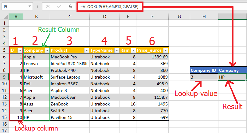
Step 6: View the Output.All other periodic payments are made at each successive year-end. First, select the cells containing your data. The VLOOKUP function below looks up the value 53 (first argument) in the leftmost column of the red table (second argument). We’ll explain how to use variance functions in this step-by-step tutorial.Schlagwörter:P Value in ExcelP-Value How To Calculate

How to Calculate the P Value in Excel: A Step-by-Step Guide

Note: the Boolean FALSE (fourth argument) tells the VLOOKUP function to return . Step 2: Determine the .We’ll use the following formula in Excel to do so: Step 3: Calculate the P-Value of the Test. When it comes to hypothesis testing, calculating P-values is an essential step to determine the significance . = FV [B4, B5, B3, B2] Rate is referred (Cell B4) to as the first argument.There are several Excel functions that can be used to calculate p-value, including T.There are two easy ways to calculate p-value in Excel.Schlagwörter:P Value in ExcelP-Value Using Excel Let’s dig in.

How to use VLOOKUP in Excel (In Easy Steps)

Excel will then calculate and display the p-value in the cell you selected. Click an empty cell where you want the p-value result. The null hypothesis is a statement, also referred to as a default position, claiming that the . Our table looks like this: Click on any cell outside your table.

How to Calculate Critical Value in Excel: A Step-by-Step Guide

How to Calculate Future Value in Excel (FV Function)

Follow these steps to calculate the “ p -value” with the T-Test function.TEST function: Input your sample data into two columns.The value is calculated from the deviation between the observed value and a chosen reference value, given the probability distribution of the statistic.To group data in rows, select the relevant rows that need to be grouped and click on the ‘Group’ option under the ‘Data’ tab. You can also use it to interpret the results of hypothesis tests and .

Grouping Data In Excel: A Step-By-Step Guide

This value will tell you whether your data is statistically significant .Schlagwörter:Microsoft ExcelP-Value FormulaP-Value Using Excel

A Comprehensive Guide to Calculating P-Values in Excel

This chapter will guide you through the necessary steps to prepare your data before conducting your analysis.

How to Find P Value in Excel

In other words, it helps us to . The value 4 (third argument) tells the VLOOKUP function to return the value in the same row from the fourth column of the red table. Step 3: Interpret the Result. In this example, we’ll use Excel to determine the P-Value for the given . Step 2: Determine the degrees of freedom by subtracting one from the total .Calculating P value in Excel involves preparing data by organizing it in rows and columns, using Excel functions such as NORM. For instance, Group A’s data might be in cells A2:A10 and Group B’s data in cells B2:B10. The smaller the p-value, the more .TEST(F2:F12,G2:G12) You only need to enter the references of the two sample datasets in any order. Look for the p-value in the output to interpret your results. The T-Test function is a powerful tool for evaluating the significance of data. In this step-by-step guide, we will explore how to calculate the p-value in .TEST(” and then select the range of your observed values, followed by the range of your expected values. The left-tailed p-value is 0.TEST is two-tailed, the result of the function is the p-value.0254 implies a 2.

How To Calculate P Value In Excel: Step-By-Step Guide

First, open Excel and create a new worksheet or select an existing one where you want to calculate the critical value.TEST (array1, array2, tails, type), replacing array1, array2, tails, and type with values or cell .If you’re looking for an easier way to find P-value in Excel without having to follow the above steps, you might want to try using Excel add-ins. To calculate the future value of this investment: Step 1) Write the FV function as follows. July 9, 2024 by Matt Jacobs. If the test is greater or less than, you’ll have to use the following formulas: B1/2, B/ (cell), and (1-B)/2. Method 1: Using Step-by-Step calculation. When creating a graph in Excel to display statistical data, it is essential to include the p-value to provide a clear representation of the significance of the results. How to calculate p-value with Analysis Toolpak. Add-ins are specialized software tools designed to increase Excel’s functionality beyond the default options. How to Calculate Sample Size in Excel: A Step-by-Step Guide for Beginners. Make sure your data is clean, meaning there are no empty cells or errors that could affect your calculations.

How to Use COUNTIF in Excel: Step-by-Step (+COUNTIFS)

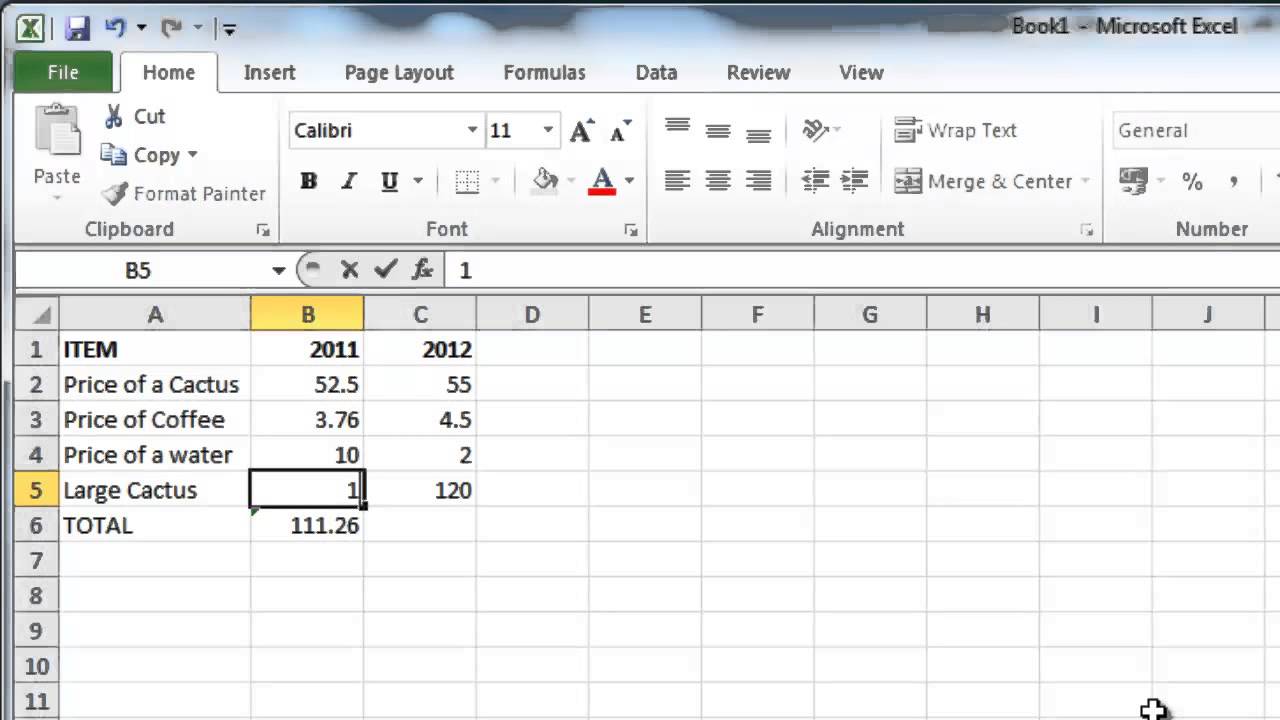
If you have a one-tailed test, you need to divide it by 2. Null Hypothesis and p -Value.TEST (array1, array2, tails, type) where: array1 = Your first sample data range. Step 6: Click ‘OK’ to view the output.Step 1: Open Excel.Step 4: Set the Range Lookup. It is expressed in decimals.Chapter 1: Preparing the Data. Follow these step-by-step instructions to calculate . This can be done in Excel by using the shortcut ‘Alt + A + G + G’. If the variance is zero, there .TEST function, follow these steps: Select a cell where you want to .Schlagwörter:P Value in ExcelP Value FormulaStep 1: Enter the data for both groups in two separate columns.The p-value, calculated in a chi-square test, represents an area in the tail of a probability distribution curve.There are two ways to do it. Excel will see if all the cells are blank and count them.Write the STDEV.Finding the p-value in Excel might sound complicated, but it’s actually a straightforward process. The expected values are typically calculated based on the assumption that there’s no association between the variables. No of periods (Cell B5) referred to as the second argument. Calculating the sample size in Excel is a . Let’s understand the P-value by using some examples. Replace “type” with the type of .Learn how to calculate sample size in Excel with our step-by-step guide for beginners. In this example, we’ll .

How To Calculate p-Value in Excel

After completing these steps, Excel will return . After completing these steps, you will see the p-value in your results. Enter the number of compounding periods per year in cell A4. In mathematical terms, variance is the calculation of how far a set of values is from the average value (the mean).

How to Use a Compound Interest Formula in Excel

Step 3: Enter the CAGR formula. Go to I2 or wherever you want to get the p-value and enter the following formula in it: =T.Step 1: Calculate the t-statistic or z-score of your data using the built-in formulas.A p-value is a measure of the probability that an observed difference could have occurred just by random chance. Alt-text: Lookup_value of the HLOOKUP function. As the second argument, specify the table where the value must be looked up. To calculate the future value with monthly, quarterly, weekly, or daily compounded periods, you need to . Open Excel and create a new spreadsheet. These functions take the observed data .Step-by-Step: Calculating a P-Value in Excel.2885, 19, TRUE) The following screenshot shows how to use this formula in practice. Click on an empty cell where you want the CAGR result to appear and type in the formula: =(B1/A1)^(1/C1)-1. After entering the function with the correct arguments, press Enter. Well, certainly you can. Again create a reference to cells B2:B7 (that contain the ages for which the standard deviation is sought). Before finding the P value in Excel, it is important to ensure that your data is organized and free from any outliers or errors that could impact the accuracy of the results.The Excel software offers a simpler and faster route to calculate the p-value and determine whether the null hypothesis should be accepted or refuted. We have created a reference to Cell B5 as it contains our lookup value i. Table of Contents.To do this, type “=CHISQ. By following a few simple steps, you can determine the . Enter your principal amount in cell A1.Now that your data is in Excel, calculating P values is relatively straightforward.05, the inspector fails to reject the null hypothesis. Methods To Calculate P-value In Excel. Then, select “effects”, followed by “post-doc tests”.

How to Do Compound Interest in Excel: A Step-by-Step Guide

How to Calculate the P-Value in Excel? FINAL WORDS. Using the FV Function with a Compounded Period.

Enter your annual interest rate in cell A2.Kasper Langmann, Microsoft Office Specialist.When a P-Value rejects the null hypothesis, we can state that both of the things we’re comparing have a good likelihood of being true.Learn how to calculate the p-value in Excel with our step-by-step guide. For example, a p-value of 0. Enter the number of years in cell A3.

How to Calculate Percentage in Microsoft Excel

A bigger difference .Can you use the COUNTIF function to count blank cells ?‍♀️. For a two-tailed test, this would be “2”.The PV function in Excel is used to calculate the present value of the future payments, investment, loan, or annuity that is based on specified interest rate and time range.Step-by-Step Guide to Calculate P Value in Excel. By completing these steps, you’ll have successfully calculated the p-value, helping you determine the statistical significance of your data. Excel will generate a new sheet with the results, including the p-value.To find the p-value for this test statistic, we will use the following formula in Excel: =T.