SIZZ

The goal is to create a cell with #N/A for every row in the column, except the last row.Here are six simple steps to create dynamic chart titles in Excel: Select the chart and click on “Chart Elements” to add or remove chart elements. In most of the cases, using Excel Table is the best way to create dynamic .

Dynamic Chart In Excel

Right click on the Combo Box control, and choose Format Control.

And, here I have a step by step guide create your first interactive chart.

Make an Interactive Chart in Excel

Ideally, there shouldn’t be any .Step #1: Create the dynamic named ranges.

Things to Remember here. Ensure your data is organized into a single column, and then select the data to create your histogram. In this section, we will teach you how to use the Key Performance Indicator (KPI) by geography for our company’s product and create an interactive map accordingly. Be the first to add your personal experience. Step 1: Create a Drop-down List.

How to Create Interactive Charts in Excel

However, the results can sometimes feel static and uninteresting.This simple process will help you turn static Excel charts into something much more dynamic. In addition to creating dynamic chart ranges, I also show you how to . Concatenate the text with the month selected: Cell Q3 = “Revenue Comparison for “&Q4The steps to make an interactive chart via dropdown lists’ are, Firstly, we will create a five rows and five columns table starting from cell B3 to F8.

To start off with, interactive charts help you neatly display massive amounts of data with only one graph: In addition, turning some chart elements from static to dynamic saves countless hours in the long run and prevents you from ever forgetting to update . For instance, in the first chart, we have entered the region as .Video ansehen12:33Join 400,000+ professionals in our courses here ? https://link.Autor: Leila GharaniSchlagwörter:Dynamic Charts in ExcelChart in ExcelExcel Dynamic Chart

Create your first interactive chart in Excel with this tutorial

Whether you’re doing it in MS Excel, Power BI or Tableau, the principles are the . Download and practice. With just a dash or two of creativity, Excel spreadsheets can go far beyond the norm, and you can create something truly engaging and presentable.

How to Create Interactive Charts with Dynamic Elements in Excel

How To Create Dynamic Map Chart in Excel [+Free Templates]

Schlagwörter:Interactive Excel ChartsMicrosoft ExcelExcel In-Cell Charts

Interactive Charts in Excel: A Quick Guide to Visualization Mastery

In this article, we’ll discuss how to create dynamic charts and reports in Excel. Using Formulas. To start with, set up the named ranges that will eventually be used as the source data for your future chart. Now we must go to “Fill” and select “Vary colors by point”.In this tutorial, we will cover the step-by-step process of creating dynamic charts in Excel, including how to set up your data and customize the chart to meet your specific needs.

How to Make a Graph in Microsoft Excel

It’s super easy with Excel dynamic arrays.Schlagwörter:Microsoft ExcelExcel How To Update A ChartMicrosoft Office

Excel Dynamic Chart with Drop-Down

Interactive charts demand data restructuring. Microsoft Excel.We’ll first select the table and then go to Insert > Column chart as shown below. Look at the example below.Schlagwörter:Interactive Excel ChartsDynamic Charts in Excelxlsx How to Create a Dynamic Map in Excel. Move and resize the chart, if necessary, to fit on the worksheet. Click “ Name Manager.Create an automatically sorted Excel bar chart that ALSO lets you hide and show categories based on a flag in the cell. Type “=” and select the cell that contains the chart title.While Excel provides a wide range of charting options, it can be challenging to create dynamic, interactive charts that engage your audience and allow them to .Schlagwörter:Chart in ExcelMicrosoft Excel Dynamic reports provide more insight than static reports as users can explore data sets in more depth.On the Excel Ribbon, click the Insert tab. Interactive and dynamic, these useful tools can aid decision-makers in a quick and easy analysis of relevant data. Ein interaktives . Create a dynamic chart legend for the forecast. Now select your data on the sheet.The easy way to make interactive and dynamic charts in Excel, rather than having to set-up a new chart every time.How to Create Dynamic Charts in Excel. These controls are . We’ll now select the points, right-click, and go to “Format data series”, as shown below. Add Slicers: Insert slicers to allow users to . Choose the right chart type. Step 2: Set up a form control. Step 2: Create a Data Retrieval Table.On the Developer tab, click Insert, then in the Form Control section of the dropdown, click on the Combo Box button (second from left in first row).

The initial chart now looks like this.So erstellen Sie einen dynamischen Diagrammbereich. Dynamic reporting involves creating reports with interactive elements that enable users to quickly and easily explore data sets and identify trends.To create the dynamic interactive chart by using a drop-down list, please do with the following steps: 1. Go to the Formulas tab. To do this, you have to make a cell reference containing the month.

How to Create Dynamic Charts in Excel Using Data Filters

For example, you want it to say, “Revenue Comparison for [month]”.Office 365 dynamic arrays. In the list of Line chart styles, click the 2-D Line option., using Excel Table and Named Ranges. After that click on “Insert” followed by “Table”.; There are two ways to create a dynamic chart, i.Learn how to create an interactive chart in Excel that switches views depending on the selection from the drop-down list.The basic steps to follow are: Create a table in Excel by selecting the table option from the Insert. Then, right click the combo box, and select Format Control from . This data is from a companies BBQ selection and they want to create a dashboard around this information. A Dialog box will appear to give the Range for the Table, and Select the option ‘ My Table has Headers . Leila Gharani shows you how to quickly create an automatically sorted Excel bar chart that ALSO lets you hide and show categories on the chart based on a flag in the cell. Based on the results displayed, we prepare a clustered column chart in excel. Draw the Combo Box, then position it where you need it.com/yt-d-all-coursesDiscover how to dynamically hide or show data series in Excel cha. TIP: Position the chart over the duplicate data range, to hide it.

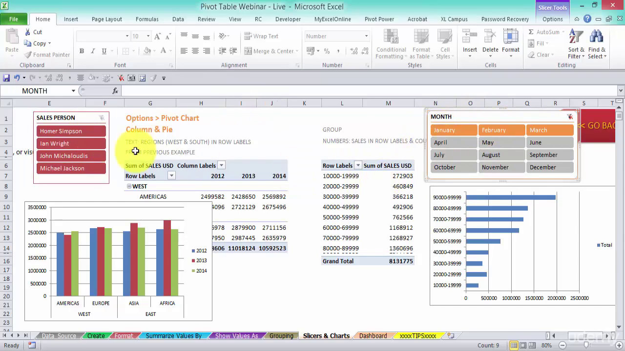
Tip: Press the F3 button to see the list of named ranges. After writing the .Create a dynamic interactive chart by using the checkboxes.To cut to the chase, just follow these simple steps to link your chart title to any cell in the spreadsheet: Click on the chart title.Need a table that updates automatically when you add new data? Create an Excel dynamic chart to keep your data consistent without extra work.Right-click on the chart and click Select Data. Step 3: Extract Data from Table 1 to Table 2. Applying a Named . Let’s consider an example of developing animations for interactive design elements in Excel data visualization.A guide on how to create dynamic charts in Excel using data filters and also without them.Step by step process Build the pivot table and charts. It shows 3 methods which uses Excel Table, Named Range, and adding Multiple Drop-down. In the dashboard sheet, add a combo-box form control (Developer Ribbon > Form Controls) and set . Customize the chart elements. Press “Enter” to complete the formula and the chart . Customer Service Dashboard. They are: Using an Excel Table.A Dynamic Chart in Excel accepts selected data modification to the existing dataset and updates the generated chart automatically. Step 4: Insert and Format . Includes practice workbook. In the New Name dialog box, create a brand new named range: Type “ Quarter ” .There are two ways to create a dynamic chart range in Excel: Using Excel Table. Click on the chart title and begin to type a formula.; An OFFSET formula works differently if there are any blank cells in the middle of the data range.So, creating interactive charts with dynamic elements allows you to kill two birds with one stone.

Advanced dynamic array formula techniques (3 methods)

The cursor turns into drawing crosshairs. Next, let’s create a dynamic label for the Forecast line.

How to Create an Interactive Excel Dashboard

Schlagwörter:Interactive Excel ChartsExcel Dynamic ChartDynamic ChartsLearn how to create a chart in Excel and add a trendline.INDEX is a function that can be used to reduce the output of our array function.Schlagwörter:Interactive Excel ChartsDynamic Charts in Excel

How to Create Dynamic Charts in Excel

The formula in cell G3 is: =INDEX(SORT(B3:E10,2,-1),{1;3;5;7},{1,4}) The SORT function is applied to cells B3-E10, in descending order based on column 2. Enter the corresponding named range after the exclamation mark. Auch hier sollten herkömmlicherweise jedes Mal, wenn Sie Elemente zum Datenbereich hinzufügen oder entfernen, der zum Erstellen eines Excel-Diagramms verwendet wird, auch die Quelldaten manuell angepasst werden. We must use form controls Form Controls Excel Form Controls are objects which can be inserted at any place in the worksheet to work with data and handle the data as specified.Creating Interactive Charts in Excel Using Dropdown Lists. We are using an Excel Table, so we must ensure our formulas react to any new data. In the group of chart types, click the Insert Line Chart command.In diesem Tutorial wird gezeigt, wie Sie interaktive Diagramme mit dynamischen Elementen in allen Excel-Versionen erstellen: 2007, 2010, 2013, 2016 und 2022. Select “Chart.To create a histogram in Excel, you’ll need to use the Histogram chart type under the Insert tab. Highlight the cell you are going to turn into your new chart title. In short: We are adding interactivity to the map. You can review recommended charts .Schlagwörter:Interactive Excel ChartsData VisualizationSchlagwörter:Chart in ExcelExcel Dynamic ChartSchlagwörter:Interactive Excel ChartsChart in ExcelExcel Dynamic Chart

How to Create Dynamic Charts With Dropdown Lists in Excel

You have the option of adding a dynamic chart header. Click in the Input Range box, .Schlagwörter:Interactive Excel ChartsDynamic Charts in Excel

Create Interactive Charts with Animated Buttons in Excel

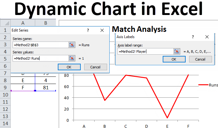
First, you should insert a drop-down list form, please click Developer > Insert > Combo Box (Form Control), and then draw a combo box as below screenshots shown: 2.How to Create a Graph or Chart in Excel.By using interactive charts in excel you can present more data in a single chart. Als nächstes: Einrichten eines dynamischen Diagrammbereichs.Choose Chart Elements as you wish to.=XLOOKUP (H3, B3:B6,C3:E6).Download Map Chart in Excel. In the Series Values box, delete the cell references but leave the worksheet name with exclamation mark (!). Select a Series item on the left box and click Edit. Firstly, open your Excel document. So, let’s look at our dataset.

How to Create a Dynamic Chart Range in Excel

Finally, the chart is a colorful one now.Create Charts: Use Excel’s charting tools to create the visual elements of your dashboard, such as bar charts, line graphs, and pie charts.Schlagwörter:Microsoft ExcelData VisualizationInteractive Graphs in Excel One way to address this problem is to add some design flourishes, but you can also introduce an interactive .

In the Name Manager dialog box that appears, select “ New. Visualize your data with a column, bar, pie, line, or scatter chart (or graph) in Office. The column chart is ready, as shown below.Create Interactive Charts with Animated Buttons in Excel. For more examples of using SORT, check out this post. Type “ = ” into the Formula Bar. Dashboard Training Course.Just add it to data model by setting up a relationship between Issue [Onwer] and People [Person]. Excel offers many types of graphs from funnel charts to bar graphs to waterfall charts.

Adding a dynamic chart title. Charts are very central when it comes to communicating information. Excel will automatically bin your data, but you can customize these settings for more precise analysis.This article shows how to make dynamic charts in Excel. Add interactivity with slicers and . The above method can only show one data series of the chart each time, if you need to show two or . There are 3 convenient ways to create dynamic charts in Excel.What are they, how to make one? Dynamic Dashboard in Excel. Specialized Chart Types: Bullet; Sales Funnel; HEAT Map; For more storytelling . But that was child’s play compared to what dynamic chart titles are truly capable of. Excel makes it easy to create clear, concise charts from your raw data.Dynamic Elements: Keep charts updated with Dynamic Chart Ranges and Titles. Excel interactive charts require advanced Excel skills.

• Gold note ph-10 im test: genialer phonoverstärker für 1.400 euro – gold note ph 10
• Metz fernseher gibt nach umzug keinen ton mehr von sich? – metz fernseher ton weg
• Soziale netzwerke: erfolgsrezepte für kmu, soziale netzwerke erfolgsrezepte
• Adrialin 2000 gaggenau | adrialin 2000
• Pourquoi et comment devenir une entreprise éco-responsable – comment être éco responsable
• Traurige songs 2024-2025 ♫ top 50 beste traurige musik 2024 _ traurige songs 2024