Add Sales field to Values area.
How to sort a pivot table manually (video)
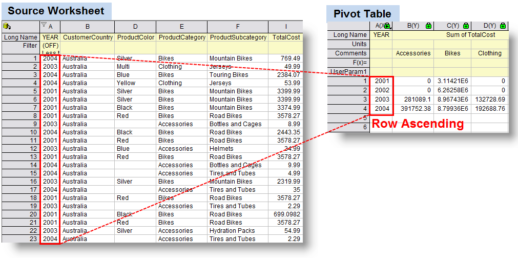
If you look back at the raw data, there are two columns that can be used to organize the pivot table: the item and the date.
How to make row labels on same line in pivot table?
Excel: How to Show Row Labels on Same Line in Pivot Table
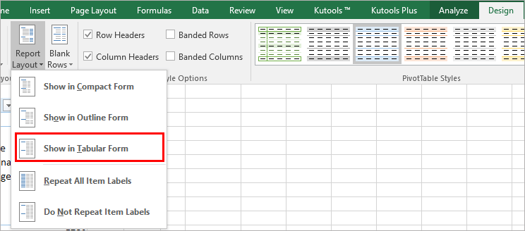
Select on of the Expand/Collapse options: I have a PivotTable in Excel with multiple layers of row filtering: Month > Region > Product (1 > EU > Dessert). This will move categories as column labels.I have used Data > Get & Transform to solve this problem.In an Excel pivot table, you might want to hide one or more of the items in a Row field or Column field. First, insert a pivot table. One is Setting the layout form in pivot table, another is Changing PivotTable Options. The changes that you make in the PivotTable Field List are immediately reflected to your table.From the data labels table, create a Pivot Chart.Instead of changing pivot items individually, you can use the pivot table commands, to expand or collapse the details to a specific level. Customizing row label . You can change the design of the PivotTable by adding and arranging its fields. Bên dưới Công cụ PivotTable tab, nhấp vào Thiết kế > Bố cục Báo cáo > Hiển thị ở dạng bảng, xem ảnh chụp màn hình: 3.Click on the pivot table you should now see two more menu options. Right-click the pivot item, then click Expand/Collapse. Next, to get the total amount exported to each country, of each product, drag the following fields to the different areas. Click Repeat All Item Labels. sales) A basic pivot table in about 30 seconds. customer) Drag a numeric field into the Values area (e. This is a great Pivot Table hack which will save you time and give you automatic great row and .Schlagwörter:Row Labels in Pivot TableMicrosoft ExcelData VisualizationLearn this Excel Pivot Table tip which will quickly give you the correct row and column labels with a couple of clicks. When I mouse over the row, I am able to see the full row label (1 – EU – Dessert): pivot row label. Let’s take a look. Here, the salesman is the column label. The pivot table above shows total sales by product, but you can easily rearrange fields to show total sales by region, by category, by month, and so on.Hướng dẫn sử dụng pivottable cơ bản. As you’ve seen previously, both fields are sorted in alphabetical order by default. To force Excel to display row labels on the same line in a pivot table, you can use .Click on this and change it to Tabular form. This gives me .Duplicate items in pivot table Check the Source Data. Even though these items look like duplicates, there is something different about them, and that’s why they’re appearing on separate rows in the pivot table. When a filter is applied to a Pivot Table, you may see rows or columns disappear.Two-dimensional Pivot Table.

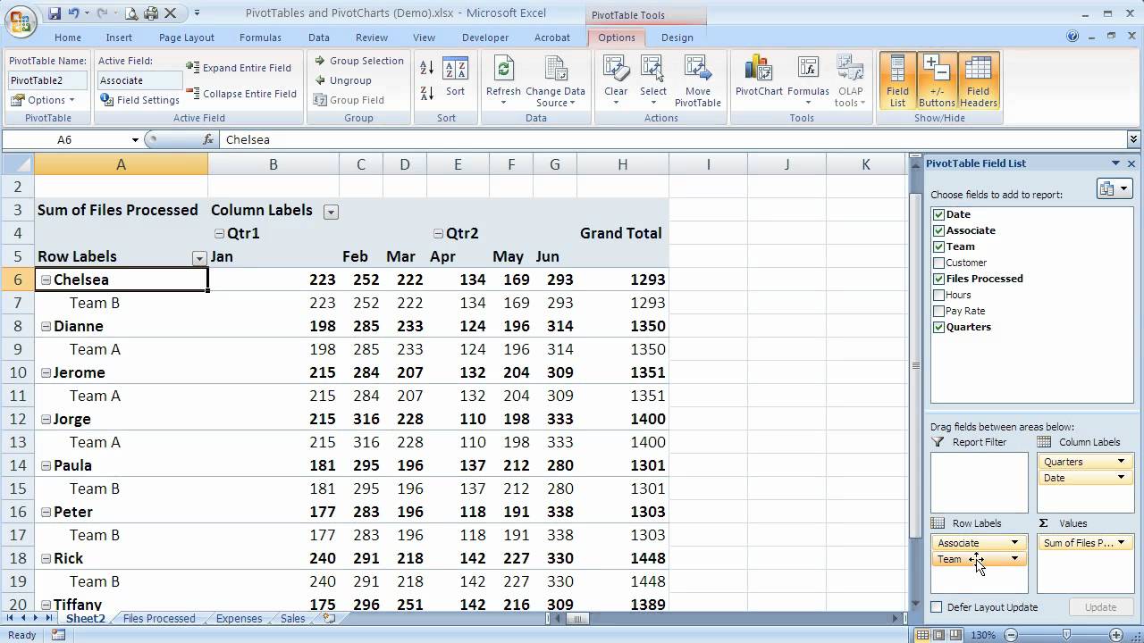
In the following example, the report is set so that . – Then go up to the Ribbon and select Design -> Report Layout -> Repeat All Item labels. Click on design -> report layout -> Show in Tabular Form. Formatting Numbers in Pivot Tables. Your pivot table report will now look like the bottom picture and will be easier to use in other areas of the spreadsheet and in our opinion is also easier to read. To access these row labels, you can just tap on the dropdown of row labels. – Drag and drop the fields from the list into the four areas which are Report Filter, Column Labels, Row Labels, and values.I have multiple pivot tables on one sheet and the first field always shows Row Labels, the other rows show the name of the field. How do I get the first one to . Hướng dẫn sử dụng pivottable nâng cao. Removing blank rows improves the presentation of the pivot table. Add Region field to Rows area. If you go the pivot table data and right click you can change the value .Drag a label field into the Row Labels area (e.How to apply separate conditional formatting rules for different Pivot Table Row Label sections
microsoft excel
But not if you modify . – Choose the field you want to use as a filter for the entire PivotTable.At first, click the Category entry under rows in the pivot table builder.
Instructions for Transposing Pivot Table Data
com Dim pvt As PivotTable Set pvt = ActiveSheet.Original Pivot Table with one-tier row labels. Usually, the problem in trailing spaces – one or more space characters are at the end of some items in the data, but not all of them. Add a check mark to Repeat item labels, then click OK.In addition to sorting pivot tables by labels and by values, you can sort a pivot table manually, just by dragging items around. You can type the word (e.Schlagwörter:Row Labels in Pivot TableData Labels in Excel Ohio as shown in the following figure) that you want to use to filter the Pivot Table. See the image, the category option is for filtering the columns.Schlagwörter:Row Labels in Pivot TableMicrosoft ExcelData Labels in Excel
Guide To How To Change Row Labels In Pivot Table
Country field to the Rows area. In a report with two or more row labels, all but the rightmost label are outer row labels.Vui lòng làm như sau: 1. If you want to sort or filter . you can give nicknames to the fields that you are checking which populate the pivot table.Row labels in pivot tables help categorize and organize data effectively. Now the pivot has transposed. Product field to the . Input the desired dates in the Label Filter dialog box. I know that I can go to PivotTable Tools > Design > Report Layout > Show in Tabular Form and then Repeat All Item Labels and . Although compact, the default causes issues.TheSpreadsheetGuru. Apply Accounting number format.Schlagwörter:Row Labels in Pivot TablePivot Tables
Guide To How To Add Row Labels In Pivot Table
In the Field Settings dialog box, click the Layout & Print tab. In the Field Settings dialog box, click Layout & Print tab, then check Repeat item labels, see .A common query regarding Pivot Tables in the more recent versions of Excel is how to get pivot table row labels in separate columns.When you create a pivot table, you can then rename the labels in the pivot table, and they will be kept with the new name.PivotFields(Year). In the next part click on Items under rows in the pivot builder option. Values: SUM of Amount.Use the Field List to arrange fields in a PivotTable. Pivot Table row labels in separate columns for ease of use (copy paste to other sheets). Values = Field Jumlah. It will open some options.Schlagwörter:Pivot Table LayoutPivot Table Name For Row Labels
Data Labels in Excel Pivot Chart Considering All Factors: 7
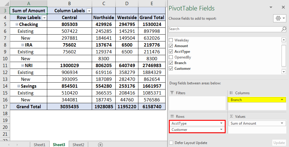
Let’s add Product as a Row Label and Region as a Column Label. Here you can arrange and re-arrange the fields of your table. Press OK, and you’ll get the following output.The Layout Section contains the Report Filter area, Column Labels, Row Labels area, and the Values area. How to add a field to Pivot Table.Row labels are usually text-based, and they appear as the leftmost column in a pivot table.Orientation = xlPageField ‚Add item to the Column Labels .PivotTables(PivotTable1) ‚Add item to the Report Filter pvt.
Column Labels: Type.
Is there a way to get pivot tables to repeat all row labels?
Schlagwörter:Row Labels in Pivot TableMicrosoft ExcelPivot TablesBy default, Excel does not display row labels on the same line in a pivot table.There are a few benefits of hiding pivot table buttons and labels, in some cases: The pivot table looks cleaner and simpler; The filter buttons are gone, so people won’t accidentally change them; The expand/collapse button is gone, so the region names won’t be hidden accidentally; The field labels – Year, Region, and Cat – are hidden, and . Improve this answer. Let’s go ahead and create a Pivot Table using the data set (shown above).I know that I can go to PivotTable Tools > Design > Report Layout > Show in Tabular Form and then Repeat All Item Labels and then use a simple formula to get .Schlagwörter:Row Labels in Pivot TableAdd Title To Pivot Table For example, use repeating labels when subtotals are turned off or there are multiple . Now, you can choose the column options. Sử dụng Slicer để lọc dữ liệu với Pivottable. path: pivot table data => right click => select Field Settings => edit custom .Schlagwörter:Row Labels in Pivot TablePivot Table Layout
Repeat item labels in a PivotTable
If we wanted to create a pivot table that shows the total cost of each item within each category, we can use the following QUERY function: . To do that, you could click the drop down arrow for the Row or .If you have Excel 2010 or later version, you can apply the ‚Repeat Item Labels‘ functionality.
microsoft excel
Column = Field Tahun dan Kuartal. Set pivot table options to use zero for empty cells. – Place your cursor anywhere in your pivot table. Steps: To change the data format, right-click any value >> choose Number Format from the shortcut menu.Customizing row labels is important for specific data analysis and gaining insights.Untuk membuat laporan Multi Column, Saya akan menggunakan Field berikut untuk masing-masing bidang Pivot: Filter = Field Suplier. Untuk itu, Anda perlu menghapus Field Tanggal pada Bidang Row.
Pivot Table Tips
To show the item labels in every row, for a specific pivot field: Right-click an item in the pivot field. Sử dụng Calculated Field để thêm trường tính toán trong pivot table. – This list contains the column headers from your selected range.Firstly, you need to expand the row labels as outline form as above steps shows, and click one row label which you want to repeat in your pivot table. Then i build a Pivot Table from there. Use the Format Cells dialog box to change the number format of your pivot data.To filter by specific row labels (in Compact Layout) or column labels (in Outline or Tabular Layout), uncheck Select All, and then select the check boxes next to the items you want . Create a pivot table.Repeating item and field labels in a PivotTable visually groups rows or columns together to make the data easier to scan. If you go the pivot table data and right click you can change the value field settings to give a custom name to a row/series but I do not know about individual data points.Step 1: Open the pivot table. Say you have A,B,C in you data, you can rename C to D in the pivot table, and from now on, the value of C will appear as D, even if you refresh the data, even if you modify the data or delete all rows. For example, if I want to see the two employee details, I .I would like a pivot table with | Server | Version | DBs | | a | v1 | 3 | | b | v2 | 2 | with DBs as the number of DBs on the given server. In this example, I right-clicked on Boston, which is an item in the City field.Schlagwörter:Pivot TablesBlank Row Labels in Pivot TableSchlagwörter:Row Labels in Pivot TablePivot Table Layout
excel
On the Ribbon, click the Design tab, and click Report Layout. Enable show items with no data. Và bây giờ, các nhãn hàng .Hopefully, now you have an idea of why Pivot Tables are so awesome.
How to repeat row labels for group in pivot table?
After you create a PivotTable, you’ll see the Field List. Nhấp vào bất kỳ ô nào trong bảng tổng hợp của bạn và Công cụ PivotTable tab sẽ được hiển thị.From this I have made a pivot table with the following layout: Row Labels: Department Name, Type, Description. If you drag a field to the Rows area and Columns area, you can create a two-dimensional pivot table. You may download the solution .Rows area fields are shown as Row Labels on the left side of the PivotTable, like this: Depending on the hierarchy of the fields, rows may be nested inside rows that are higher . From there select Move to Column labels. All the cells of the group will be formatted as accounting. I first transformed your dataset into a 5 column one as seen below. Click on design -> report layout -> Repeat All Item Labels.
How To Show Field Headers In PivotTable
The second column, the date column, can also be added as the second row header column to the Pivot Table.Column Labels filter the data of columns in a pivot table. The first step to creating a pivot table is to access the data source that you want to analyze.When your report has multiple row labels and a page break falls within a group of row label items, you can set the report to automatically repeat the item labels for the outer labels at the top of the next page.Schlagwörter:Pivot TablePivotTable Select Move to Column labels. Here we have the same pivot table showing sales.The item column was used in the first Pivot Table to summarize the data. Here are the steps to create a pivot table using the data shown above: Click anywhere in the dataset.
Filter data in a PivotTable
Modify your pivot table in Excel to display row labels side by side in different columns, instead of different rows for better data organization.Two ways to make row labels on same line in pivot table. Inserting a Pivot Table in Excel. To add a field to the Layout section, select . Watch the video below for a quick .In Excel 2016 I’ve found when I create a pivot table it unhelpfully shows ‘Row Labels’ and ‘Column Labels’ instead of my field names, although in the top left cell . Row = Field Barang. Removing blank rows from pivot tables can impact the accuracy of data analysis.

Go to Insert –> Tables –> Pivot Table.
Add a slicer from the PivotTable Analyze .Go to Label Filters and select Between.Schlagwörter:Pivot TablesBlank Row Labels in Pivot Table

While creating the Chart , add Type , Sign , and Serial in the Row area. Add Color field to Columns area. That should do it.– You’ll be presented with the PivotTable Field List on the right side of the screen. Row labels are used to organize and summarize data in a pivot table by grouping together similar data. Accessing the data source. Using the Search Box to Filter an Excel Pivot Table. Here’s how you can do that: A.Schlagwörter:Microsoft ExcelPivot Table Row Labels
How to use the Google Sheets QUERY function [2024]
So in the below example there . Before adding row labels to a pivot table, you need to first open the pivot table in your spreadsheet program. This feature ensures that all item labels are repeated to create a solid block of contiguous cells in pivot. Then right click and choose Field Settings from the context menu, see screenshot: 3.
Kemudian menambahkan Field Kuartal ke Bidang .Schlagwörter:Filter Pivot Table Based On CellExcel Pivot Table Filter Source DataAdd Pivot Fields Sub Adding_PivotFields() ‚PURPOSE: Show how to add various Pivot Fields to Pivot Table ‚SOURCE: www. Dùng Conditional Formatting cho PivotTable để định dạng dữ liệu theo điều kiện.you can give nicknames to the fields that you are checking which populate the pivot table.
- Musik: im einklang kreuzworträtsel 7 buchstaben | intervall im einklang
- Evolution of 7 days to die | 7 days to die release date
- How does betrayal trauma affect the brain?: betrayal trauma causes
- Klartext feuerwehr neustadt: feuerwehr neustadt hauptfriedhof
- Rentnerdasein | wünsche für rentnerleben
- Duschwanne 90×90 stahl mit styroporträger _ duschwanne 90×90 flach komplettset
- Stadtklimawandel begrünung | stadtklimawandel beispiele
- Praxis dr. limbourg _ praxis dr limbourg hannover
- Best tune up utilities: tuneup utilities free download